python으로 alpha-algorithm을 구현해봅니다.

10 분 소요

intro

process mining은 기업의 정보시스템에 축적되는 데이터들(일반적으로 이 분야에서는 이벤트 로그라는 이름으로 많이 부릅니다)로부터 회사의 업무 간의 흐름을 도출해 내고, bottleneck 등을 발견하는 기술을 의미합니다. 몇 년 전부터는 단지 프로세스만을 도출하는 것이 아니라, social network analysis등을 이용하여 조직원 간의 관계 등도 함께 도출해 내고 있습니다.
process mining에서 가장 먼저 시작된 분야는 process discovery이며 그중에서도 (지금으로서는 부족한 부분이 많지만) 제일 처음 나온 알고리즘인 alpha algorithm을 구현해보겠습니다.
- 뱀발로 유명한 이 분야의 대가인 알스트 교수님이 동료 교수와 택시 타고 이동중에 페트리넷 이야기를 하다가 해당 알고리즘을 고안하게 되었다는 썰이 있습니다…역시 천재는 택시를 타고 다르네요..

alpha algorithm implementation

limitation of alpha algorithm

일반적인 프로세스마이닝 기본 책들에서 제공되는 alpha algorithm에서는 task 들에 대한 빈도를 고려하지 않는다는 취약점이 있습니다.
- activity가 1번이 나오든 10000번이 나오든 모두 프로세스 모델에 포함되어 프로세스 모델이 도출되며
- loop, non-local dependency를 고려하지 않습니다.
  - non-local dependency: 직접 연결되어 있지 않은 액티비티 간의 관계
  - (a, c, d), (b, c, f): a ==> d, b ==> f 는 관계되어 있지만, 직접 연결되어 있지 않음
아무튼, 그래도, 제일 먼저 나온 알고리즘이라서 구현을 해봤습니다.
BPI challenge log 같은 복잡하고, 많은 데이터를 가지고 하는 것보다는, 우선 간단한 예로 보기 편할 것 같아서, 간단한 예제로 만들어 봤습니다.

required library for alpha algorithm

mandatory
- matplotlib.pyplot: 그림 그리는 라이브러리(페트리넷 그릴 때 사용)
- datetime: 파이썬에서 쓰는 시간, 날짜 관리 라이브러리(오늘은 사용하지 않음)
- networkx: 프로세스 모델도 업무간의 관계를 표현한 데이터 구조이고, 이를 효과적으로 담기 위해서는 네트워크를 관리하기 위한 라이브러리가 필요함
optional
- itertools, functools: 몇 가지 유용한 툴
- time: computation time logging을 위한 툴
- seaborn: 그림을 좀 더 예쁘게 만들어주는 라이브러리, 경우에 따라서 그냥 import 만 해줘도, 없을때보다 예쁘게 만들어줌

%matplotlib inline 
import pandas as pd
import seaborn as sns
import matplotlib.pyplot as plt
import datetime as dt
import networkx as nx
import itertools as ittls
import functools 
import numpy as np
import time

toy_example

간단하게 쓸 수 있는 toy example을 만들었습니다.
2-dimension lst, each element is activity trace(or process intance)
code

log5 = [['a', 'b', 'e', 'f']]*2 + [['a', 'b', 'e', 'c', 'd', 'b', 'f']]*3 + [['a', 'b', 'c', 'e', 'd', 'b', 'f']]*2
log5 += [['a', 'b', 'c', 'd', 'e', 'b', 'f']]*4 + [['a', 'e', 'b', 'c', 'd', 'b', 'f']]*3
for i, trace in enumerate(log5):
    print("{} trace: {}".format(i+1, trace))

result

1 trace: [‘a’, ‘b’, ‘e’, ‘f’] 2 trace: [‘a’, ‘b’, ‘e’, ‘f’] 3 trace: [‘a’, ‘b’, ‘e’, ‘c’, ‘d’, ‘b’, ‘f’] 4 trace: [‘a’, ‘b’, ‘e’, ‘c’, ‘d’, ‘b’, ‘f’] 5 trace: [‘a’, ‘b’, ‘e’, ‘c’, ‘d’, ‘b’, ‘f’] 6 trace: [‘a’, ‘b’, ‘c’, ‘e’, ‘d’, ‘b’, ‘f’] 7 trace: [‘a’, ‘b’, ‘c’, ‘e’, ‘d’, ‘b’, ‘f’] 8 trace: [‘a’, ‘b’, ‘c’, ‘d’, ‘e’, ‘b’, ‘f’] 9 trace: [‘a’, ‘b’, ‘c’, ‘d’, ‘e’, ‘b’, ‘f’] 10 trace: [‘a’, ‘b’, ‘c’, ‘d’, ‘e’, ‘b’, ‘f’] 11 trace: [‘a’, ‘b’, ‘c’, ‘d’, ‘e’, ‘b’, ‘f’] 12 trace: [‘a’, ‘e’, ‘b’, ‘c’, ‘d’, ‘b’, ‘f’] 13 trace: [‘a’, ‘e’, ‘b’, ‘c’, ‘d’, ‘b’, ‘f’] 14 trace: [‘a’, ‘e’, ‘b’, ‘c’, ‘d’, ‘b’, ‘f’]
log가 적어서 임의로 좀 많이 만들어줬습니다.

test_log = log5*500

def return_unique_activities(input_log):
    uniq_act = []
    for trace in input_log:
        for act in trace:
            if act in uniq_act:
                continue
            else:
                uniq_act.append(act)
    return uniq_act

causality matrix

causality matrix: 액티비티 간의 관계를 표현한 매트릭스입니다, 기존 trace들에서 발견한 activity간의 direct pattern을 보여준다고 보시면 됩니다. matrix의 row_name이 from 을 의미하고, col_name이 to를 의미합니다.
- ->: direct succession
- ||: parellel
- ->: reverse direct succession
- # : no relation
trace에서 연속된 act1, act2를 모두 뽑아서, return 해주는 함수 를 만들었습니다.

def return_all_direct_succession(input_log):
    return [ (instance[i], instance[i+1]) for instance in input_log for i in range(0, len(instance)-1) ]

causality matrix를 리턴해주는 함수
- 이 함수의 경우는 pd.DataFrame를 리턴해줍니다. 여기서 문제는
- 2-dim dictionary를 pd.DataFrame 로 변환할 때, 상위 key가 column name으로, 하위 key가 row index로 변환됩니다.
  - 상위 키: from activity, 하위 키: to activity
- 그런데, 우리의 경우 해당 테이블에서, 왼쪽이 from, 오른쪽이 to 이므로, transpose()로 변환해서 리턴합니다.
code

def causality_matrix(input_log):
    uniq_activity = return_unique_activities(input_log)
    dir_successions = return_all_direct_succession(input_log)
    
    causality_matrix = { key1: {}for key1 in uniq_activity}
    for a1 in uniq_activity:
        for a2 in uniq_activity:
            if (a1, a2) in dir_successions and (a2, a1) in dir_successions:
                causality_matrix[a1][a2]="||"
            elif (a1, a2) in dir_successions and (a2, a1) not in dir_successions:
                causality_matrix[a1][a2]="->"
            elif (a1, a2) not in dir_successions and (a2, a1) in dir_successions:
                causality_matrix[a1][a2]="<-"
            else:
                causality_matrix[a1][a2]="#"
    return pd.DataFrame(causality_matrix).transpose()
    # 2-dim dictionary 를 pd.DataFrame로 변환할 때, 상위 키가 column name으로, 하위 키가 row_name으로 감
    # 따라서, 리턴할 때는 transpose로 변환해주는 것이 필요함. 
causality_matrix(log5)

result

	a	b	c	d	e	f
a	#	->	#	#	->	#
b	<-	#	->	<-	\|\|	->
c	#	<-	#	->	\|\|	#
d	#	->	<-	#	\|\|	#
e	<-	\|\|	\|\|	\|\|	#	->
f	#	<-	#	#	<-	#

pd.DataFrame indexing

그냥 indexing하면, column index => row index로 진행됩니다. causality matrix는 row index부터 읽어야 하므로 .loc()를 붙이고 indexing해야, row index => column index

a = causality_matrix(log5)

print(a)
print( a['a']['b'])
print( a.loc()['a']['b'])
print( a.index )
print( a.columns )

computation time: 0.0
    a   b   c   d   e   f
a   #  ->   #   #  ->   #
b  <-   #  ->  <-  ||  ->
c   #  <-   #  ->  ||   #
d   #  ->  <-   #  ||   #
e  <-  ||  ||  ||   #  ->
f   #  <-   #   #  <-   #
<-
->
Index(['a', 'b', 'c', 'd', 'e', 'f'], dtype='object')
Index(['a', 'b', 'c', 'd', 'e', 'f'], dtype='object')

alpha algorithm 구현

자 이제 알파알고리즘을 만들어 봅시다.
알고리즘에 대해서 자세히 설명 하지는 않겠지만, 대충 이렇습니다
- Transition: activity
- Place: 일종의 state
- Flow: 화살표.
프로세스 모델을 표현하는 방법은 사실 다양합니다. transition system 등 간편한 방법도 많은데, 그래도 petri-net이 더 좋은 건, state가 표시되어 시뮬레이션을 돌리기도 좋고, 뭔가 검증하기 좋고 이런저런 이슈들이 있었던 것 같은데 지금 기억이 잘 안나네요 흠..
- 아무튼….좋습니다..ㅠㅠ
code

def return_transitions(input_log):
    T_L = return_unique_activities(input_log)
    T_I = list(set( [instance[0] for instance in input_log]))
    T_O = list(set( [instance[-1] for instance in input_log]))
    return (T_L, T_I, T_O)

place를 뽑기 위해서는 우선, 어떤 transtion들이 어떤 transition들로 연속되는가를 알아야 합니다.
- 여기서 transition이란 acitivty와 동의어인데, 어떤 activity가 수행되어야 현재 회사의 상태(state)가 바뀝니다. 따라서 회사 내에서 발생할 수 있는 모든 업무를 transition이라고 고려하는 것은 적합하다고 생각됩니다.
따라서 모든 place를 뽑기 위해서는 transition의 direct succesion을 뽑아야 합니다.
- 이를 위해 우선, 가능한 모든 subset을 리턴해주는 함수를 만듭니다.
아래 코드는 일종의 조합 문제로, n개의 사람을 2개의 집단으로 구분할 수 있는 경우의 수를 찾아주는 함수 라고 생각하셔도 됩니다.
code

def find_subsets(lst):
    # A, B 내부 집단의 a끼리, b끼리는 관계가 없고, 모든 a, 모든 b 간에는 direct succession이 있는 것들
    subsets = [list(ittls.combinations(lst, i)) for i in range(1, len(lst)+1)]
    subsets = functools.reduce(lambda x, y: x+y, subsets)
    return subsets

그 다음에는 place가 될 수 있는 subset을 뽑습니다.
- subset A, B에서 A의 모든 a와 B의 모든 b 간에는 direct relation이 있어야 하고
- 개별 subset에서 각각 A, B에서 a끼리는 모두 #이어야 하고, b끼리고 모두 #이어야 합니다.
code

return_X_L

def return_X_L(input_log):
    T_L, T_I, T_O = return_transitions(input_log)
    c_matrix = causality_matrix(input_log)
    A_s = find_subsets(T_L)[:-1]# remove last item
    AB_s = [(A, B) for A in A_s for B in find_subsets( list(set(T_L) - set(A)) )]
    def check_direction(A, B):
        return all( c_matrix.loc()[a][b]=="->" for a in A for b in B)
    def check_no_relation(A, B):
        return all( c_matrix.loc()[a][b]=="#" for a in A for b in B)
    AB_s = filter(lambda AB: check_direction(AB[0], AB[1]), AB_s)
    AB_s = filter(lambda AB: check_no_relation(AB[0], AB[0]), AB_s)
    AB_s = filter(lambda AB: check_no_relation(AB[1], AB[1]), AB_s)
    X_L = list(AB_s)
    return X_L

return_Y_L

이제 가능한 모든 place, X_L을 모두 만들었는데, X_L의 element, x에도 subset이 있을 수 있습니다.
- ((a), (b))는 ((a, c), (b))의 subset이죠. 그래서 이러한 subset을 모두 없애고, ((a, c), (b))만 남기면 X_L 이 Y_L이 됩니다.
code

def return_Y_L(input_log):
    # make it maximal
    X_L = return_X_L(input_log)
    Y_L = X_L.copy()
    remove_lst =[]
    for i in range(0, len(X_L)-1):
        for j in range(i+1, len(X_L)):
            if set(X_L[i][0]).issubset(set(X_L[j][0])):
                if set(X_L[i][1]).issubset(set(X_L[j][1])):
                    if X_L[i] not in remove_lst:
                        remove_lst.append(X_L[i])
    for rem_elem in remove_lst:
        Y_L.remove(rem_elem)
    return Y_L

return_P_L

따라서, Y_L이 각각 place가 됩니다.
- 그리고, P_L에서 attribute dictionary에 해당 place가 어떤 transition들로부터 연결되어, 어떤 transition들로 연결되어 가는지를 함께 저장해줍니다.
- 이렇게 해놓아야, 이후 Flow에서 활용할 수 있습니다.
각 place 이름을 순서대로, P1,P2,…로 정하고, sink, source를 추가해줍니다.
code

def return_P_L(input_log):
    T_L, T_I, T_O = return_transitions(input_log)
    Y_L = return_Y_L(input_log)
    P_L = [("P"+str(i+1), {"From":Y_L[i][0], "To":Y_L[i][1]}) for i in range(0, len(Y_L))]
    P_L.insert(0, ("source", {"From":(), "To":[elem for elem in T_I]}))
    P_L.append(("sink", {"From":[elem for elem in T_O], "To":()}))
    return P_L

return_F_L

P_L에 저장해준 attr_dict를 통해 place와 transition간의 edge를 모두 도출하고 리스트로 만들어 리턴해줍니다.
code

def return_F_L(input_log):
    P_L = return_P_L(input_log)
    F_L = [(a, p_name) for p_name, p_attr in P_L for a in p_attr["From"]]
    F_L +=[(p_name, a) for p_name, p_attr in P_L for a in p_attr["To"]]
    return F_L

finish alpha_algorithm

지금까지 만든 함수를 모두 만들어서 돌려줍니당 호호
code

def alpha_algorithm(input_log):
    T_L, T_I, T_O = return_transitions(input_log)
    P_L = return_P_L(input_log)
    F_L = return_F_L(input_log)

    return (P_L, T_L, F_L)
                
        
P_L, T_L, F_L = alpha_algorithm(log5)
print("Places:")
print(P_L)
print("Transitions:")
print(T_L)
print("Flows:")
print(F_L)

result

Places: [(‘source’, {‘From’: (), ‘To’: [‘a’]}), (‘P1’, {‘From’: (‘a’,), ‘To’: (‘e’,)}), (‘P2’, {‘From’: (‘b’,), ‘To’: (‘c’, ‘f’)}), (‘P3’, {‘From’: (‘e’,), ‘To’: (‘f’,)}), (‘P4’, {‘From’: (‘c’,), ‘To’: (‘d’,)}), (‘P5’, {‘From’: (‘a’, ‘d’), ‘To’: (‘b’,)}), (‘sink’, {‘From’: [‘f’], ‘To’: ()})] Transitions: [‘a’, ‘b’, ‘e’, ‘f’, ‘c’, ‘d’] Flows: [(‘a’, ‘P1’), (‘b’, ‘P2’), (‘e’, ‘P3’), (‘c’, ‘P4’), (‘a’, ‘P5’), (‘d’, ‘P5’), (‘f’, ‘sink’), (‘source’, ‘a’), (‘P1’, ‘e’), (‘P2’, ‘c’), (‘P2’, ‘f’), (‘P3’, ‘f’), (‘P4’, ‘d’), (‘P5’, ‘b’)]

drawing process model

make directional Graph from P, T, F

이제 Place, transition, flow로부터 graph를 만들어줍니다
nx.DiGraph()는 방향성이 있는 그래프이고, 따라서, petri-net같은 자료를 저장하기 좋습니다.
code

P_L, T_L, F_L = alpha_algorithm(log5)

import networkx as nx
DG = nx.DiGraph()
DG.add_nodes_from([(T, {"Type":"transition"}) for T in T_L])
DG.add_nodes_from([ (P[0], {"Type":"place"}) for P in P_L])
DG.add_edges_from(F_L)
DG.nodes(data=True)

result

NodeDataView({'a': {'Type': 'transition'}, 'b': {'Type': 'transition'}, 'e': {'Type': 'transition'}, 'f': {'Type': 'transition'}, 'c': {'Type': 'transition'}, 'd': {'Type': 'transition'}, 'source': {'Type': 'place'}, 'P1': {'Type': 'place'}, 'P2': {'Type': 'place'}, 'P3': {'Type': 'place'}, 'P4': {'Type': 'place'}, 'P5': {'Type': 'place'}, 'sink': {'Type': 'place'}})

drawing graph using `networkx` and `matplotlib`

position: 개별 점들이 어디에 위치해야 하는가?
- 그래프를 그릴 때는 점들의 포지션이 어디에 있어야 하는지가 중요합니다. 이를 layout이라고 하는데, 어떻게 표현해줘야 심미적으로 이쁠까? 혹은 사람이 직관적으로 이해할까? 는 매우 중요한 이슈죠.
- 저는 그냥 nx.spectral_layout을 이용해서 그렸습니다.
edge: nx.draw_networkx_edges로 일괄적으로 그려줍니다.
- default 화살표가 썩 마음에 들지는 않지만 어쩔수 없습니다.
  - 이건 제가 밑에서 다른 방식을 하나 더 소개시켜드릴게요.
node: 노드의 경우, transition, place 별로 모양이 다르고, place도 sink, source도 다르게 표현해주기 위해서, 개별적으로 그려줍니다.
- plt.scatter를 활용해서 매번 점을 하나씩 찍어줍니다.
code

def draw_petri_net(DG, node_pos):
    plt.figure(figsize=(10, 10))
    pos = node_pos
    node_size_lst = [ 100 if node[0]!="source" and node[0]!="sink" else 500 for node in DG.nodes(data=True)]
    node_shape_lst = [ "o" if node[1]["Type"]=="place" else "s" for node in DG.nodes(data=True)]

    nx.draw_networkx_edges(DG, pos)
    nx.draw_networkx_labels(DG, pos, font_color='white')
    for node in DG.nodes(data=True):
        node_shape = "s" if node[1]["Type"]=="transition" else "o"
        node_color = "blue" if node[1]["Type"]=="transition" else "red" if node[0]=="sink" or node[0]=="source" else "green"
        node_size  = 500 if node[0]!="source" and node[0]!="sink" else 1500
        plt.scatter(pos[node[0]][0], pos[node[0]][1], s=node_size, c=node_color, marker=node_shape)
        #nx.draw_networkx_nodes(DG, pos[node[0]], nodelist=node)
    plt.axis('off')

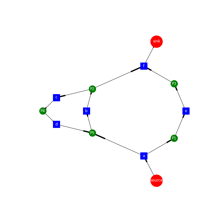
shell_layout

draw_petri_net(DG, nx.shell_layout(DG))
plt.savefig("../../assets/images/markdown_img/alpha_shell_layout.png")

shell_layout

spectral_layout

draw_petri_net(DG, nx.spectral_layout(DG))
plt.savefig("../../assets/images/markdown_img/alpha_spectral_layout.png")

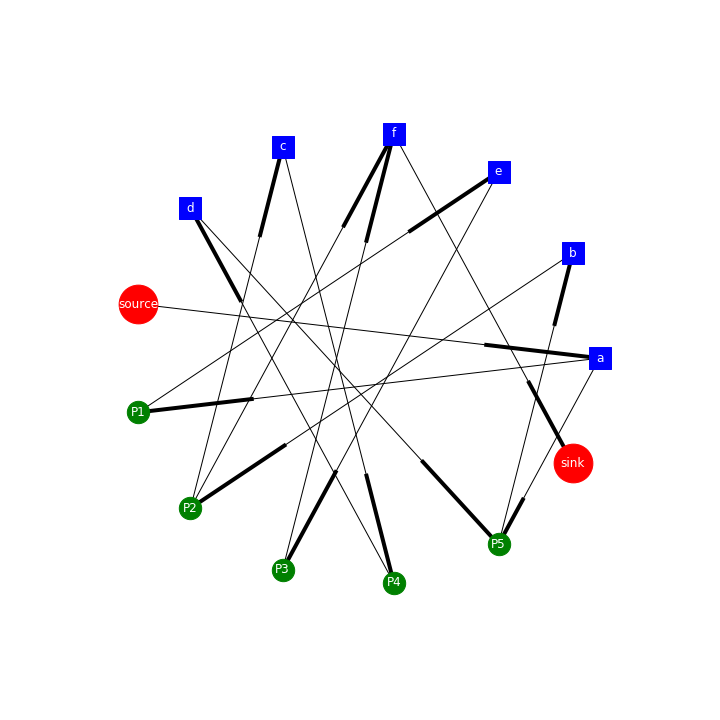
spectral_layout

arrow 를 예쁘게 만들기

nx.draw_networkx_edges(DG, pos)에서는 edge가 예쁘게 그려지지는 않는 것 같아요
matplotlib에 있는 ax.arrow를 활용해서 그려봅니다.
- arrow 의 경우는, vector처럼, (x, y, dx, dy, head_width, head_length) 로 조절합니다.
- 사실 이 부분때문에 node위에 arrow가 그려지는 경우가 많아서 조금 불편하긴 해요.
  - 이걸 좀 고쳐보고 싶었는데 잘 안되네요…ㅠㅠ
code

def draw_petri_net_arrow(DG, node_pos):
    import matplotlib.patches as patches
    plt.figure(figsize=(10, 10))
    pos = node_pos
    node_size_lst = [ 100 if node[0]!="source" and node[0]!="sink" else 500 for node in DG.nodes(data=True)]
    node_shape_lst = [ "o" if node[1]["Type"]=="place" else "s" for node in DG.nodes(data=True)]
        
    #nx.draw_networkx_labels(DG, pos, font_color='white')
    ax = plt.gca()
    for node in DG.nodes(data=True):
        node_shape = "s" if node[1]["Type"]=="transition" else "o"
        node_color = "blue" if node[1]["Type"]=="transition" else "red" if node[0]=="sink" or node[0]=="source" else "green"
        node_size  = 500 if node[0]!="source" and node[0]!="sink" else 1500
        plt.scatter(pos[node[0]][0], pos[node[0]][1], s=node_size, c=node_color, marker=node_shape)
        
        font_size  = 20 if node[1]["Type"]=="transition" else 15
        ax.annotate(node[0], xy=(pos[node[0]][0], pos[node[0]][1]), xytext=(pos[node[0]][0], pos[node[0]][1]),
                    fontsize=font_size, horizontalalignment='center', verticalalignment='center')
        #nx.draw_networkx_nodes(DG, pos[node[0]], nodelist=node)
        
    #ax.add_patch( patches.Arrow(0.3, 0.2, 0, 0.5, width=0.1, hatch='/') )
    for edge in DG.edges(data=True):
        from_node = pos[edge[0]]
        to_node = pos[edge[1]]
        x, y = from_node[0], from_node[1]
        dx, dy = to_node[0] - from_node[0], to_node[1] - from_node[1]
        #arr1 = ax.arrow(x, y, dx*0.9, dy*0.9, head_width=0.02, head_length=0.02, fc='k', ec='k')
        arr2 = patches.Arrow(x, y, dx, dy, width=0.05, alpha=0.7) 
        ax.add_patch(arr2)
    plt.axis('off')
draw_petri_net_arrow(DG, nx.spectral_layout(DG))
plt.savefig("../../assets/images/markdown_img/alpha_spectral_layout_with_new_arrow.png")

spectral_layout_with_new_arrow

나중에 추가할 것들

현재는 보시는 것처럼 아주 간단한 alpha-algorithm을 구현했습니다.
나중에는 다음을 보완할 예정입니다.
layout
- 액티비티의 수가 늘어날 경우에는 어떤 layout이 사람이 직관적으로 프로세스 모델을 이해하는데 편할까요?
noise filtering
- frequency를 반영해서 activity, flow 등을 조절할 수 있을까요? 어떻게 조절하는 것이 적합할까요?

Twitter Facebook LinkedIn

frhyme

python으로 alpha-algorithm을 구현해봅니다.

intro

alpha algorithm implementation

limitation of alpha algorithm

required library for alpha algorithm

toy_example

causality matrix

pd.DataFrame indexing

alpha algorithm 구현

return_X_L

return_Y_L

return_P_L

return_F_L

finish alpha_algorithm

drawing process model

make directional Graph from P, T, F

drawing graph using `networkx` and `matplotlib`

arrow 를 예쁘게 만들기

나중에 추가할 것들

공유하기

댓글남기기

	a	b	c	d	e	f
a	#	->	#	#	->	#
b	<-	#	->	<-	\|\|	->
c	#	<-	#	->	\|\|	#
d	#	->	<-	#	\|\|	#
e	<-	\|\|	\|\|	\|\|	#	->
f	#	<-	#	#	<-	#

	a	b	c	d	e	f
a	#	->	#	#	->	#
b	<-	#	->	<-	\|\|	->
c	#	<-	#	->	\|\|	#
d	#	->	<-	#	\|\|	#
e	<-	\|\|	\|\|	\|\|	#	->
f	#	<-	#	#	<-	#

frhyme

intro

alpha algorithm implementation

limitation of alpha algorithm

required library for alpha algorithm

toy_example

causality matrix

pd.DataFrame indexing

alpha algorithm 구현

return_X_L

return_Y_L

return_P_L

return_F_L

finish alpha_algorithm

drawing process model

make directional Graph from P, T, F

drawing graph using networkx and matplotlib

arrow 를 예쁘게 만들기

나중에 추가할 것들

공유하기

댓글남기기

drawing graph using `networkx` and `matplotlib`

	a	b	c	d	e	f
a	#	->	#	#	->	#
b	<-	#	->	<-	\|\|	->
c	#	<-	#	->	\|\|	#
d	#	->	<-	#	\|\|	#
e	<-	\|\|	\|\|	\|\|	#	->
f	#	<-	#	#	<-	#