keras의 model을 파봅시다.
model class가 뭔가요.
- 저는 지금까지 keras를 이용해서, neural network를 설계할 때,
Sequential을 사용했습니다. 어차피 제가 만드는 뉴럴넷 모델들은 그저 선형적으로 쭉 이어져 내려올 뿐이었거든요(mnist를 이용한 image classification, 기본적인 RNN 등) - 그런데, 지난번에 GAN을 간단하게 만들어보고, 쭉 보니까, 복잡한 모델들이 매우 많은 것 같아요. 예를 들면
- 이미 만든 모델에서 일정 부분만 가져와서 새로운 모델 만들기
- 이미 만든 모델들을 합쳐서 새로운 모델 만들기
- 이런걸 원활하게 해주려면 keras의
modelclass를 알아야 하는 것 같아요. 이미 ‘학습한’ 모델을 재사용하고 싶을때, 그럴때 model을 사용하는 것 같습니다. 일단은 이정도만 알고, keras의 documentation을 확인해보면서 진행해보도록 하겠습니다.
make NN by Sequential
- 일단은 sequential model부터 다시 복습해보겠습니다. 레이어들이 그냥 일렬로 쭉 나열된 형태죠.
Sequential이Model과 다른 것은, 모델의 맨 앞에Input가 없다는 것이죠.Sequential의 경우, 첫번째 레이어에서input_shape에 input의 데이터 형태를 함께 넘겨줍니다.
#### data reading
from tensorflow.examples.tutorials.mnist import input_data

mnist = input_data.read_data_sets("MNIST_data/", one_hot=True)
x_train, y_train = mnist.train.images, mnist.train.labels
x_test, y_test = mnist.test.images, mnist.test.labels

from keras.models import Sequential, Model
from keras.layers import Input, Dense, Activation
from keras.optimizers import Adam, SGD
from keras import metrics

## sequential model
seq_model = Sequential([
    Dense(512, input_shape=(784,), activation='relu'),
    Dense(128, activation='relu'),
    Dense(32, activation='relu'),
    Dense(10, activation='softmax'),
])

print("#### Sequential Model")
seq_model.summary()
seq_model.compile(loss='categorical_crossentropy',
              optimizer=Adam(lr=0.001, beta_1=0.9, beta_2=0.999, epsilon=1e-8),
              metrics=[metrics.categorical_accuracy])
train_history = seq_model.fit(x_train, y_train, epochs=5, batch_size=500, verbose=2)
train_history = train_history.history # epoch마다 변화한 loss, metric

loss_and_metric = seq_model.evaluate(x_train, y_train, batch_size=128, verbose=0)
print("train, loss and metric: {}".format(loss_and_metric))
loss_and_metric = seq_model.evaluate(x_test, y_test, batch_size=128, verbose=0)
print("test, loss and metric: {}".format(loss_and_metric))
- input layer가 없습니다.
Extracting MNIST_data/train-images-idx3-ubyte.gz
Extracting MNIST_data/train-labels-idx1-ubyte.gz
Extracting MNIST_data/t10k-images-idx3-ubyte.gz
Extracting MNIST_data/t10k-labels-idx1-ubyte.gz
#### Sequential Model
_________________________________________________________________
Layer (type)                 Output Shape              Param #
=================================================================
dense_74 (Dense)             (None, 512)               401920
_________________________________________________________________
dense_75 (Dense)             (None, 128)               65664
_________________________________________________________________
dense_76 (Dense)             (None, 32)                4128
_________________________________________________________________
dense_77 (Dense)             (None, 10)                330
=================================================================
Total params: 472,042
Trainable params: 472,042
Non-trainable params: 0
_________________________________________________________________
Epoch 1/5
5s - loss: 0.4589 - categorical_accuracy: 0.8673
Epoch 2/5
4s - loss: 0.1492 - categorical_accuracy: 0.9570
Epoch 3/5
5s - loss: 0.0983 - categorical_accuracy: 0.9716
Epoch 4/5
5s - loss: 0.0712 - categorical_accuracy: 0.9784
Epoch 5/5
5s - loss: 0.0515 - categorical_accuracy: 0.9844
train, loss and metric: [0.041054270681467921, 0.98849090910824866]
test, loss and metric: [0.078584650909528139, 0.97660000000000002]
make NN by Model
Sequential이 아닌Model을 사용하여 뉴럴넷을 설계합니다. 차이는 앞서 말씀드린 대로,Input이 있는 경우와 없는 경우로 구분이 되겠죠.Model은 input, output만 넣어줍니다.
- 앞서 만든
seq_model의 레이어를 직접 가져와서 거의 그대로 설계 했습니다. - 또한, 레이어를 가져오는 것은 물론이고 바로 뒤에
argument가 함께 들어가 있어야 합니다. 아래 코드를 보시면 연속적으로 input2, nD1, …, nD3 이런식으로 바로바로 이전 레이어가 다음 레이어의 input으로 들어가 있는 것을 알 수 있습니다. - 약간 이 부분이 이해가 좀 안되기는 하는데, 일단 그냥 넘어가겠습니다.
- 이전 뉴럴넷이 새롭게 컴파일 되지 않는 한, 이전 뉴럴넷이 다시 fitting을 하여 parameter들이 변화했다면, 아래 레이어들에서도 값이 변화합니다. 단
compile을 새롭게 하게 되면, 뉴럴넷 자체를 새롭게 구성하겠다는 말이므로, 분화된 레이어를 가지게 됩니다.
input2 = Input(shape=(784,))
nD1 = seq_model.layers[0](input2)
nD2 = seq_model.layers[1](nD1)
nD3 = seq_model.layers[2](nD2)
nD4 = seq_model.layers[3](nD3)
model1 = Model(input2, nD4) # input, output
model1.compile(loss='categorical_crossentropy',
              optimizer=Adam(lr=0.001, beta_1=0.9, beta_2=0.999, epsilon=1e-8),
              metrics=[metrics.categorical_accuracy])
model1.summary()

loss_and_metric = model1.evaluate(x_train, y_train, batch_size=128, verbose=0)
print("train, loss and metric: {}".format(loss_and_metric))
loss_and_metric = model1.evaluate(x_test, y_test, batch_size=128, verbose=0)
print("train, loss and metric: {}".format(loss_and_metric))
_________________________________________________________________
Layer (type)                 Output Shape              Param #
=================================================================
input_35 (InputLayer)        (None, 784)               0
_________________________________________________________________
dense_74 (Dense)             (None, 512)               401920
_________________________________________________________________
dense_75 (Dense)             (None, 128)               65664
_________________________________________________________________
dense_76 (Dense)             (None, 32)                4128
_________________________________________________________________
dense_77 (Dense)             (None, 10)                330
=================================================================
Total params: 472,042
Trainable params: 472,042
Non-trainable params: 0
_________________________________________________________________
train, loss and metric: [0.041054270681467921, 0.98849090910824866]
train, loss and metric: [0.078584650909528139, 0.97660000000000002]
multi-input and multi-output
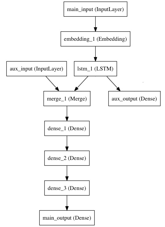
- 여러 input과 output이 함께 들어오는 뉴럴넷을 설계해보겠습니다. 앞서 본 것과 같이,
Sequential로는 이러한 형태를 만드는 것이 조금 어려운 것 같아요. 제가 참고한 포스트에 있는 내용을 그대로 활용하여 아래 그림과 같은 뉴럴넷을 만들어 보겠습니다.- fitting까지는 하지 않습니다.
- 코드는 사실 제가 참고한 keras documentation에 있는 내용들과 동일합니다.
- 몇 가지 포인트라면,
- multi input은
keras.layers.concatenate를 이용해서 합침 - multi input/output은 fitting할 때, name을 key로 넘겨줘야 함. 따라서 name을 명확하게 명시할 것.
- multi input은
import keras
from keras.layers import Input, Embedding, LSTM, Dense
from keras.models import Model

# Headline input: meant to receive sequences of 100 integers, between 1 and 10000.
# Note that we can name any layer by passing it a "name" argument.
main_input = Input(shape=(100,), dtype='int32', name='main_input')

# This embedding layer will encode the input sequence
# into a sequence of dense 512-dimensional vectors.
x = Embedding(output_dim=512, input_dim=10000, input_length=100)(main_input)

# A LSTM will transform the vector sequence into a single vector,
# containing information about the entire sequence
lstm_out = LSTM(32)(x)

auxiliary_output = Dense(1, activation='sigmoid', name='aux_output')(lstm_out)

auxiliary_input = Input(shape=(5,), name='aux_input')
#######################
#### concatenate inputs
x = keras.layers.concatenate([lstm_out, auxiliary_input])

# We stack a deep densely-connected network on top
x = Dense(64, activation='relu')(x)
x = Dense(64, activation='relu')(x)
x = Dense(64, activation='relu')(x)

# And finally we add the main logistic regression layer
main_output = Dense(1, activation='sigmoid', name='main_output')(x)

model = Model(inputs=[main_input, auxiliary_input], outputs=[main_output, auxiliary_output])

model.compile(optimizer='rmsprop', loss='binary_crossentropy',
              loss_weights=[1., 0.2])
"""
model.fit({'main_input': headline_data, 'aux_input': additional_data},
          {'main_output': labels, 'aux_output': labels},
          epochs=50, batch_size=32)
"""
model.summary()
____________________________________________________________________________________________________
Layer (type)                     Output Shape          Param #     Connected to
====================================================================================================
main_input (InputLayer)          (None, 100)           0
____________________________________________________________________________________________________
embedding_3 (Embedding)          (None, 100, 512)      5120000     main_input[0][0]
____________________________________________________________________________________________________
lstm_3 (LSTM)                    (None, 32)            69760       embedding_3[0][0]
____________________________________________________________________________________________________
aux_input (InputLayer)           (None, 5)             0
____________________________________________________________________________________________________
concatenate_2 (Concatenate)      (None, 37)            0           lstm_3[0][0]
                                                                   aux_input[0][0]
____________________________________________________________________________________________________
dense_85 (Dense)                 (None, 64)            2432        concatenate_2[0][0]
____________________________________________________________________________________________________
dense_86 (Dense)                 (None, 64)            4160        dense_85[0][0]
____________________________________________________________________________________________________
dense_87 (Dense)                 (None, 64)            4160        dense_86[0][0]
____________________________________________________________________________________________________
main_output (Dense)              (None, 1)             65          dense_87[0][0]
____________________________________________________________________________________________________
aux_output (Dense)               (None, 1)             33          lstm_3[0][0]
====================================================================================================
Total params: 5,200,610
Trainable params: 5,200,610
Non-trainable params: 0
____________________________________________________________________________________________________
- summary보다는 그림이 좀 더 보기 편합니다.
from IPython.display import SVG #jupyter notebook에서 보려고
from keras.utils.vis_utils import model_to_dot # keras model을 dot language로 변환
from keras.utils import plot_model

plot_model(model1, to_file='../../assets/images/markdown_img/180624_nn_multi_in_output.svg')
SVG(model_to_dot(model, show_shapes=True).create(prog='dot', format='svg'))

wrap-up
- 뭐, 뒤에 몇 가지 내용들이 더 있긴 합니다만, 일단은 이정도로만 하려고 합니다.
- 지금까지는, Sequential만을 이용해서 그냥 만들었는데, 가능하면,
Model로Input까지 함께 정의해주는 것이 좀 더 좋은 습관인 것 같고, - 이미 만들어진 Model의 layer들을 활용하거나, 분화해서 새로운 모델을 만들 수 있다(특히 학습된 parameter들이 있기 때문에).
- 정도가 좋은 내용인 것 같아요. 나머지는 제가 encoder, decoder를 활용해서 좀 더 써먹어보겠습니다.
댓글남기기